Learning Molecular Representation using Graph Neural Network - Molecular Graph

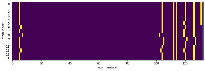
Taking a look at how graph neural network operate for molecular representations

Motivation

I have used chemprop previously and got interested in how it works internally. I’ve read their papers several times, but I’m not a machine learning researcher, and how it handles the molecular reprentation using the graph neural network was not entirely clear to me. So, here I’ll spend some time going through their code and try to understand it my own way. Most of the code was initially taken from the chemprop repository and I striped away the parts that I don’t need for clarity.

%matplotlib inline
import matplotlib.pyplot as plt
import matplotlib

from io import BytesIO
import pandas as pd
import numpy as np
from IPython.display import SVG

# RDKit 
import rdkit
from rdkit.Chem import PandasTools
from rdkit import Chem
from rdkit.Chem import AllChem
from rdkit.Chem import DataStructs
from rdkit.Chem import rdMolDescriptors
from rdkit.Chem import rdRGroupDecomposition
from rdkit.Chem.Draw import IPythonConsole #Needed to show molecules
from rdkit.Chem import Draw
from rdkit.Chem import rdDepictor
from rdkit.Chem.Draw import rdMolDraw2D
from rdkit.Chem.Draw.MolDrawing import MolDrawing, DrawingOptions #Only needed if modifying defaults

DrawingOptions.bondLineWidth=1.8
IPythonConsole.ipython_useSVG=True
from rdkit import RDLogger
RDLogger.DisableLog('rdApp.warning')
print(rdkit.__version__)

# pytorch
import torch
from torch.utils.data import DataLoader, Dataset, Sampler
from torch import nn

2020.03.2

Message passing neural network (MPNN)

Chemprop adopts a variant of graph neural network called “directed message passing neural network (D-MPNN)”. Let’s first talk about MPNN and discuss the difference between the MPNN and D-MPNN later.

MPNN is a model that operates on an undirected graph, G with a set of nodes v and edges e. This is appealing because molecules can be thought as a graph with nodes (atoms) and edges (bonds).

MPNN operates in two phases; molecular encoding phase and the feed-forward phase (the paper uses “message passing phase” and “readout phase”, respectively). In the molecular encoding phase, the features in the atoms and bonds are passed around T times to build a molecular representation of the molecule and the molecular properties are predicted in the feed-forward phase. The parameter T is also called “depth” and represents how “far” each nodes can “see”.

Compared to a typical MPNN, the package chemprop adopts directed MPNN (D-MPNN) architecture using bond features. Although the molecular graph does not have a direction, one can treat each bond as two directed edges that goes opposite direction. One of the advantage of this approach is to prevent totters (message that goes back to itself because the first node is the its neighbor of neighbor). chemprop also uses bond feature, which is concatenated feature vector of atom and bond feature vectors.

Let’s take a look at how chemprop featurizes atom and bond:

Atom Features

# we will define a class which holds various parameter for D-MPNN
class TrainArgs:
    smiles_column = None
    no_cuda = False
    gpu = None
    num_workers = 8
    batch_size = 50
    atom_descriptors = None
    no_cache_mol = False
    dataset_type = 'regression'
    task_names = []
    seed = 0
    atom_messages = False
    hidden_size = 300
    bias = False
    depth = 3
    dropout = 0.0
    undirected = False
    aggregation = 'mean'
    aggregation_norm = 100

    @property
    def device(self) -> torch.device:
        """The :code:`torch.device` on which to load and process data and models."""
        if not self.cuda:
            return torch.device('cpu')

        return torch.device('cuda', self.gpu)

    @device.setter
    def device(self, device: torch.device) -> None:
        self.cuda = device.type == 'cuda'
        self.gpu = device.index

    @property
    def cuda(self) -> bool:
        """Whether to use CUDA (i.e., GPUs) or not."""
        return not self.no_cuda and torch.cuda.is_available()

    @cuda.setter
    def cuda(self, cuda: bool) -> None:
        self.no_cuda = not cuda
        
args = TrainArgs()

For atom and bond features, we can take a look at the atom_features and bond_features function below. For example, the atom feature vector consists of one-hot encoding of atomic number, degree, formal charge, chirality, number of hydrogens, and hybridization. And the bond feature vector consists of one-hot encoding of bond type (single, double, triple, aromatic) and whether the bond is conjugated or not and whether in the ring or not.

# Atom feature sizes
MAX_ATOMIC_NUM = 100
ATOM_FEATURES = {
    'atomic_num': list(range(MAX_ATOMIC_NUM)),
    'degree': [0, 1, 2, 3, 4, 5],
    'formal_charge': [-1, -2, 1, 2, 0],
    'chiral_tag': [0, 1, 2, 3],
    'num_Hs': [0, 1, 2, 3, 4],
    'hybridization': [
        Chem.rdchem.HybridizationType.SP,
        Chem.rdchem.HybridizationType.SP2,
        Chem.rdchem.HybridizationType.SP3,
        Chem.rdchem.HybridizationType.SP3D,
        Chem.rdchem.HybridizationType.SP3D2
    ],
}

# Distance feature sizes
PATH_DISTANCE_BINS = list(range(10))
THREE_D_DISTANCE_MAX = 20
THREE_D_DISTANCE_STEP = 1
THREE_D_DISTANCE_BINS = list(range(0, THREE_D_DISTANCE_MAX + 1, THREE_D_DISTANCE_STEP))

# len(choices) + 1 to include room for uncommon values; + 2 at end for IsAromatic and mass
ATOM_FDIM = sum(len(choices) + 1 for choices in ATOM_FEATURES.values()) + 2
EXTRA_ATOM_FDIM = 0
BOND_FDIM = 14


def get_atom_fdim():
    """Gets the dimensionality of the atom feature vector."""
    return ATOM_FDIM + EXTRA_ATOM_FDIM

def get_bond_fdim(atom_messages=False):
    """Gets the dimensionality of the bond feature vector.
    """
    return BOND_FDIM + (not atom_messages) * get_atom_fdim()

def onek_encoding_unk(value: int, choices: List[int]):
    encoding = [0] * (len(choices) + 1)
    index = choices.index(value) if value in choices else -1
    encoding[index] = 1

    return encoding

def atom_features(atom: Chem.rdchem.Atom, functional_groups: List[int] = None):
    """Builds a feature vector for an atom.
    """
    features = onek_encoding_unk(atom.GetAtomicNum() - 1, ATOM_FEATURES['atomic_num']) + \
               onek_encoding_unk(atom.GetTotalDegree(), ATOM_FEATURES['degree']) + \
               onek_encoding_unk(atom.GetFormalCharge(), ATOM_FEATURES['formal_charge']) + \
               onek_encoding_unk(int(atom.GetChiralTag()), ATOM_FEATURES['chiral_tag']) + \
               onek_encoding_unk(int(atom.GetTotalNumHs()), ATOM_FEATURES['num_Hs']) + \
               onek_encoding_unk(int(atom.GetHybridization()), ATOM_FEATURES['hybridization']) + \
               [1 if atom.GetIsAromatic() else 0] + \
               [atom.GetMass() * 0.01]  # scaled to about the same range as other features
    if functional_groups is not None:
        features += functional_groups
    return features

def bond_features(bond: Chem.rdchem.Bond):
    """Builds a feature vector for a bond.
    """
    if bond is None:
        fbond = [1] + [0] * (BOND_FDIM - 1)
    else:
        bt = bond.GetBondType()
        fbond = [
            0,  # bond is not None
            bt == Chem.rdchem.BondType.SINGLE,
            bt == Chem.rdchem.BondType.DOUBLE,
            bt == Chem.rdchem.BondType.TRIPLE,
            bt == Chem.rdchem.BondType.AROMATIC,
            (bond.GetIsConjugated() if bt is not None else 0),
            (bond.IsInRing() if bt is not None else 0)
        ]
        fbond += onek_encoding_unk(int(bond.GetStereo()), list(range(6)))
    return fbond

Let’s take a look at the example molecule and how atom and bond features actually look like:

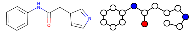
# example molecule
smiles = 'c1ccccc1NC(=O)CC1cncc1'
mol = Chem.MolFromSmiles(smiles)
mol

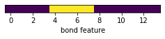
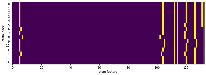
Below is the feature vector of the every atoms in the molecule. The first 100 elements represents the atomic number, followed by one hot encodings of degree (2), formal charge (0), chiral (false), total number of Hs (1), hybridization (SP2), aromaticity (1). Finally atomic mass (multiplied by 0.01) at the last entry.

feats = []
indices = []
for i in range(mol.GetNumAtoms()):
    atom = mol.GetAtomWithIdx(i)
    feat = atom_features(atom)
    feats.append(feat)
    indices.append(i)

fig = plt.figure(figsize=(12, 0.25 * mol.GetNumAtoms()))
ax = fig.add_subplot(111)
im = ax.imshow(feats, interpolation='None', cmap='viridis', aspect='auto')
plt.xlabel('atom feature')
plt.ylabel('atom index')

ax.set_yticks(indices)
ax.set_yticklabels(indices)
ax.tick_params(left=False)  # remove the ticks
plt.show()

The atom index 0 and 7 are very similar since they are both carbon atoms and only slightly different in terms of aromaticity and the number of hydrogens attached. Let’s take a look at the features of atom 0 and 7 side by side so we can see the difference more clearly.

import svgutils.compose as sc
import svgutils.transform as sg
from ipywidgets import interact, interactive, fixed
from IPython.display import SVG
from io import BytesIO

atom1 = mol.GetAtomWithIdx(0)
atom2 = mol.GetAtomWithIdx(7)
feat1 = feats[0]
feat2 = feats[7]

# draw molecule with highlight
d = rdMolDraw2D.MolDraw2DSVG(200, 150)
rdMolDraw2D.PrepareAndDrawMolecule(d, mol, highlightAtoms=(atom1.GetIdx(), atom2.GetIdx()))
d.FinishDrawing()
mol_svg = d.GetDrawingText()

# draw feature
fig = plt.figure(figsize=(3, 0.91), dpi=150)
ax = fig.add_subplot(111)
im = ax.imshow([feat1, feat2], interpolation='nearest', cmap='viridis', aspect='auto')
plt.xlabel('atom feature')
ax.set_yticks([0, 1])
ax.set_yticklabels([atom1.GetIdx(), atom2.GetIdx()])
img = BytesIO()
plt.tight_layout()
plt.savefig(img, transparent=True, format='svg')
plt.close(fig)
feat_svg = img.getvalue().decode()

# arrange figures
fig1 = sg.fromstring(mol_svg)
fig2 = sg.fromstring(feat_svg)
plot1 = fig1.getroot()
plot2 = fig2.getroot()
plot1.moveto(10, -40)
plot2.moveto(0, 65)

svg = sc.Figure("16cm", "6cm", 
        plot1.scale(0.05), 
        plot2.scale(0.05), 
      ).tostr()
SVG(svg)

# interactive plot does not work in the final page
#

import svgutils.compose as sc
import svgutils.transform as sg
from ipywidgets import interact, interactive, fixed
from IPython.display import SVG
from io import BytesIO

def drawit(m, atomId=0):
    atom = m.GetAtomWithIdx(atomId)
    feat = atom_features(atom)
    
    # draw molecule with highlight
    d = rdMolDraw2D.MolDraw2DSVG(200, 150)
    rdMolDraw2D.PrepareAndDrawMolecule(d, m, highlightAtoms=(atom.GetIdx(),))
    d.FinishDrawing()
    mol_svg = d.GetDrawingText()
    
    # draw feature
    fig = plt.figure(figsize=(3, 0.8), dpi=150)
    ax = fig.add_subplot(111)
    im = ax.imshow([feat], interpolation='nearest', cmap='viridis', aspect='auto')
    plt.xlabel('atom feature')
    ax.set_yticks([])
    img = BytesIO()
    plt.tight_layout()
    plt.savefig(img, transparent=True, format='svg')
    plt.close(fig)
    feat_svg = img.getvalue().decode()
    
    # arrange figures
    fig1 = sg.fromstring(mol_svg)
    fig2 = sg.fromstring(feat_svg)
    plot1 = fig1.getroot()
    plot2 = fig2.getroot()
    plot1.moveto(10, -40)
    plot2.moveto(0, 65)

    svg = sc.Figure("16cm", "6cm", 
            plot1.scale(0.05), 
            plot2.scale(0.05), 
          ).tostr()
    return SVG(svg)
    
interact(drawit, m=fixed(mol), atomId=(0, mol.GetNumAtoms()-1));

Bond Features

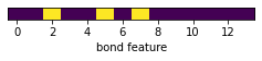
The bond feature is even more simpler. The bond feature vector consists of one-hot encoding of bond type (single, double, triple, aromatic) and whether the bond is conjugated or not and whether in the ring or not.

def bond_features(bond: Chem.rdchem.Bond):
"""Builds a feature vector for a bond.
"""
if bond is None:
    fbond = [1] + [0] * (BOND_FDIM - 1)
else:
    bt = bond.GetBondType()
    fbond = [
        0,  # bond is not None
        bt == Chem.rdchem.BondType.SINGLE,
        bt == Chem.rdchem.BondType.DOUBLE,
        bt == Chem.rdchem.BondType.TRIPLE,
        bt == Chem.rdchem.BondType.AROMATIC,
        (bond.GetIsConjugated() if bt is not None else 0),
        (bond.IsInRing() if bt is not None else 0)
    ]
    fbond += onek_encoding_unk(int(bond.GetStereo()), list(range(6)))
return fbond

# example molecule
smiles = 'c1ccccc1NC(=O)CC1cncc1'
mol = Chem.MolFromSmiles(smiles)

# let's take a look at the first bond
bond1 = mol.GetBondWithIdx(0) # C=C aromatic bond
assert bond1.GetBeginAtom().GetSymbol() == 'C'
assert bond1.GetEndAtom().GetSymbol() == 'C'

feat1 = bond_features(bond1)
assert feat1[4] == 1 # aromatic
assert feat1[6] == 1 # ring

# highlight which bond with Idx 0
d = rdMolDraw2D.MolDraw2DSVG(300, 150)
rdMolDraw2D.PrepareAndDrawMolecule(d, mol, highlightBonds=(0,))
d.FinishDrawing()
svg = d.GetDrawingText()
SVG(svg)

fig = plt.figure(figsize=(4, 0.2))
ax = fig.add_subplot(111)
im = ax.imshow(np.array(feat1)[np.newaxis, :], interpolation='None', cmap='viridis', aspect='auto')
plt.xlabel('bond feature')

ax.set(yticklabels=[])
ax.tick_params(left=False)  # remove the ticks
plt.show()

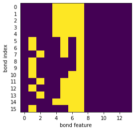
Above is the feature vector of the 0th bond. This bond is aromatic, conjugated, and in a ring. Let’s take a look at another bond feature and see how it is different from the 0th bond feature vector.

# highlight which bond with Idx 0
d = rdMolDraw2D.MolDraw2DSVG(300, 150)
rdMolDraw2D.PrepareAndDrawMolecule(d, mol, highlightBonds=(7,))
d.FinishDrawing()
svg = d.GetDrawingText()
SVG(svg)

bond2 = mol.GetBondWithIdx(7) # C=C aromatic bond
feat2 = bond_features(bond2)

fig = plt.figure(figsize=(4, 0.2))
ax = fig.add_subplot(111)
im = ax.imshow(np.array(feat2)[np.newaxis, :], interpolation='None', cmap='viridis', aspect='auto')
plt.xlabel('bond feature')

ax.set(yticklabels=[])
ax.tick_params(left=False)  # remove the ticks
plt.show()

Now you can see this bond is double bond, conjugated, and not in a ring. Let’s display the bond feature vectors of every chemical bond in the molecule.

feats = []
indices = []
for i in range(mol.GetNumBonds()):
    bond = mol.GetBondWithIdx(i)
    feat = bond_features(bond)
    feats.append(feat)
    indices.append(i)

fig = plt.figure(figsize=(4, 0.25 * mol.GetNumBonds()))
ax = fig.add_subplot(111)
im = ax.imshow(feats, interpolation='None', cmap='viridis', aspect='auto')
plt.xlabel('bond feature')
plt.ylabel('bond index')

ax.set_yticks(indices)
ax.set_yticklabels(indices)
ax.tick_params(left=False)  # remove the ticks
plt.show()

Graph featurizaation

chemprop defines the molecular graph as the code shown below. The MolGraph itself is pretty straightforward; iterates over atoms and bonds and stores atom feature and bond feature vectors into f_atoms and f_bonds attributes and construct neighboring atom indices.

class MolGraph:
    def __init__(self, mol, atom_descriptors=None):
        # Convert SMILES to RDKit molecule if necessary
        if type(mol) == str:
            mol = Chem.MolFromSmiles(mol)

        self.n_atoms = 0  # number of atoms
        self.n_bonds = 0  # number of bonds
        self.f_atoms = []  # mapping from atom index to atom features
        self.f_bonds = []  # mapping from bond index to concat(in_atom, bond) features
        self.a2b = []  # mapping from atom index to incoming bond indices
        self.b2a = []  # mapping from bond index to the index of the atom the bond is coming from
        self.b2revb = []  # mapping from bond index to the index of the reverse bond

        # Get atom features
        self.f_atoms = [atom_features(atom) for atom in mol.GetAtoms()]
        if atom_descriptors is not None:
            self.f_atoms = [f_atoms + descs.tolist() for f_atoms, descs in zip(self.f_atoms, atom_descriptors)]

        self.n_atoms = len(self.f_atoms)

        # Initialize atom to bond mapping for each atom
        for _ in range(self.n_atoms):
            self.a2b.append([])

        # Get bond features
        for a1 in range(self.n_atoms):
            for a2 in range(a1 + 1, self.n_atoms):
                bond = mol.GetBondBetweenAtoms(a1, a2)

                if bond is None:
                    continue

                f_bond = bond_features(bond)
                self.f_bonds.append(self.f_atoms[a1] + f_bond)
                self.f_bonds.append(self.f_atoms[a2] + f_bond)

                # Update index mappings
                b1 = self.n_bonds
                b2 = b1 + 1
                self.a2b[a2].append(b1)  # b1 = a1 --> a2
                self.b2a.append(a1)
                self.a2b[a1].append(b2)  # b2 = a2 --> a1
                self.b2a.append(a2)
                self.b2revb.append(b2)
                self.b2revb.append(b1)
                self.n_bonds += 2

Let’s take a look at the atom and the bond features it builds internally. The atom features are exactly same as what we discussed in the previous section.

smiles = 'c1ccccc1NC(=O)CC1cncc1'
mol = Chem.MolFromSmiles(smiles)
mol_graph = MolGraph(smiles)

# atom features
fig = plt.figure(figsize=(12, 4))
ax = fig.add_subplot(111)
im = ax.imshow(mol_graph.f_atoms, interpolation='None', cmap='viridis', aspect='auto')

ax.set_yticks(list(range(mol_graph.n_atoms)))
ax.set_yticklabels(list(range(mol_graph.n_atoms)))
ax.tick_params(left=False)  # remove the ticks
plt.xlabel('atom feature')
plt.ylabel('atom index')
plt.show()

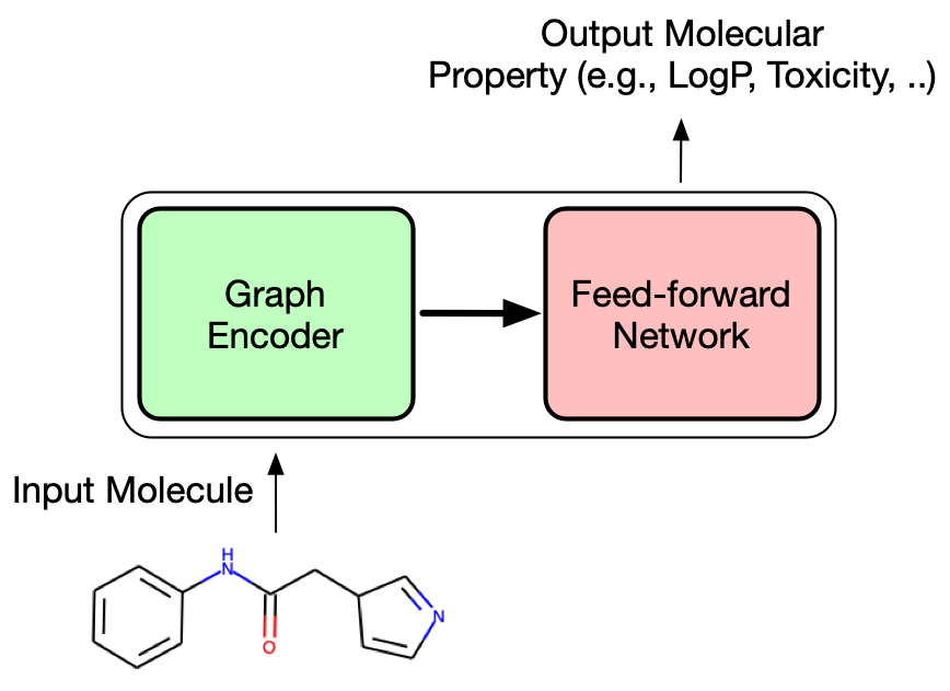
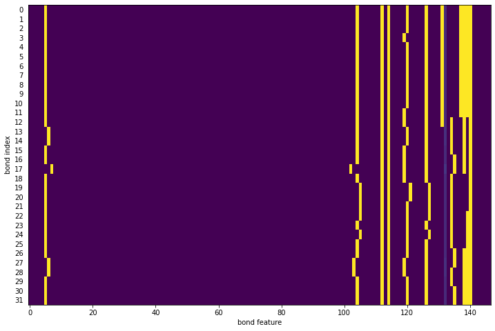
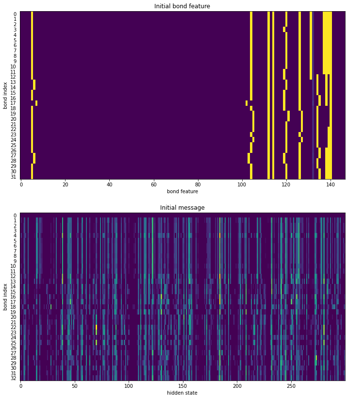
The “bond” in the molecular graph represents directed bonds. For example, there are two bonds, b1 and b2 between the atoms a1 and a2. The bond b1 is a bond from the atom a1 to atom a2 and the bond b2 is a bond from the atom a2 to a1. The bond feature is then constructed by concatenate the incoming atom (originating atom) feature and the bond feature.

# bond features : atom feature + bond feature
# bond features are added as nested atoms loop. 
# For each bond, a1->a2 and a2->a1 are added. So, more bond features than NumBonds
fig = plt.figure(figsize=(12, 8))
ax = fig.add_subplot(111)
im = ax.imshow(mol_graph.f_bonds, interpolation='None', cmap='viridis', aspect='auto')

ax.set_yticks(list(range(mol_graph.n_bonds)))
ax.set_yticklabels(list(range(mol_graph.n_bonds)))
ax.tick_params(left=False)  # remove the ticks
plt.xlabel('bond feature')
plt.ylabel('bond index')
plt.show()

The attributes a2b, b2a, and b2revb contains various mapping of atom index to bond indices, bond index to atom index, and reverse bond index. These are required for the message passing to work properly.

Message passing

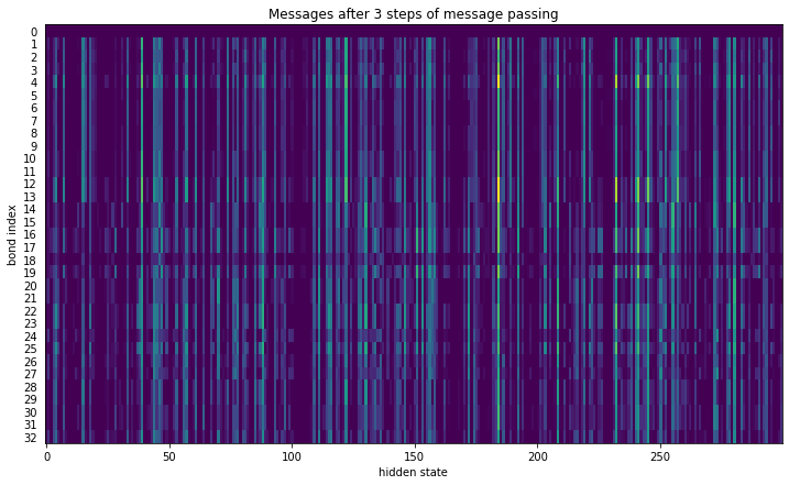
Now we are ready to dig into the most interesting part of MPNN architecture. The messages are passed around according to the connectivity, and the message evolves as it travels around the nodes.

The message passing phase consists of T steps of update cycles. In each step t, hidden state hidden state h_{vw}^t and message m_{vw}^t are updated using message function M_t and vertex update function U_t. Each message and hidden states are associated with nodes v and w. Note the direction of message matters, so h_{vw}^t and m_{vw}^t are different from h_{wv}^t and m_{wv}^t.

m_v^{t+1} = \large\sum_{k\in\{N(v)w\}}^{} M_t(x_v, x_w, h_{kv}^t)

h_{vw}^{t+1} = U_t(h_{vw}^t, m_{vw}^{t+1})

The initial hidden state for each node is defined as

h_{vw}^0 = \tau (W_i \mathrm{cat} (x_v, e_{vw}))

where W_i is a learned matrix (\mathbb{R}^{h \times h_i}), \mathrm{cat} (x_v, e_{vw}) is the concatenation of atom features (\mathbb{R}^{h_i}), x_v and the bond feature e_{vw} for bond vw, and the \tau is the activation function.

chemprop uses very simple message passing function and edge update function:

M_t(x_v, x_w, h_{vw}^t) = h_{vw}^t

U_t(h_{vw}^t, m_{vw}^{t+1}) = U(h_{vw}^t, m_{vw}^{t+1}) = \tau (h_{vw}^0 + W_m m_{vw}^{t+1}).

The W_m is a learned matrix (\mathbb{R}^{h \times h})

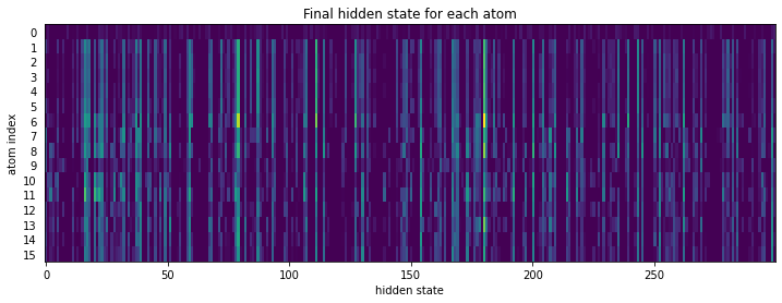
Finally, the atom representation of molecule is computed by summing over all incoming bond features.

m_v = \sum_{k \in N(v)} h_{kv}^t

h_v = \tau(W_a \mathrm{cat} (x_v, m_v))

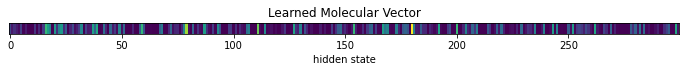
where W_a is a learned matrix (\mathbb{R}^{h \times h}). The readout phase of the D-MPNN uses the readout function, R, which is a simple summation of all the atom hidden states, which subsequently used in a feed-forward network for predicting the molecular properties.

h = \sum_{v\in G} h_v

Let’s get into to the code and see how above is implemented.

Initial message

The initial hidden state for each node is defined as

h_{vw}^0 = \tau (W_i \mathrm{cat} (x_v, e_{vw}))

# prepare the tensors for message passing
bond_fdim = get_bond_fdim()
atom_fdim = get_atom_fdim()
n_atoms = 1  # number of atoms (start at 1 b/c need index 0 as padding)
n_bonds = 1  # number of bonds (start at 1 b/c need index 0 as padding)

a_scope = []  # list of tuples indicating (start_atom_index, num_atoms) for each molecule
b_scope = []  # list of tuples indicating (start_bond_index, num_bonds) for each molecule

# All start with zero padding so that indexing with zero padding returns zeros
f_atoms = [[0] * atom_fdim]  # atom features
f_bonds = [[0] * bond_fdim]  # combined atom/bond features
a2b = [[]]   # mapping from atom index to incoming bond indices
b2a = [0]    # mapping from bond index to the index of the atom the bond is coming from
b2revb = [0] # mapping from bond index to the index of the reverse bond

f_atoms.extend(mol_graph.f_atoms)
f_bonds.extend(mol_graph.f_bonds)

for a in range(mol_graph.n_atoms):
    a2b.append([b + n_bonds for b in mol_graph.a2b[a]])

for b in range(mol_graph.n_bonds):
    b2a.append(n_atoms + mol_graph.b2a[b])
    b2revb.append(n_bonds + mol_graph.b2revb[b])

a_scope.append((n_atoms, mol_graph.n_atoms))
b_scope.append((n_bonds, mol_graph.n_bonds))
n_atoms += mol_graph.n_atoms
n_bonds += mol_graph.n_bonds

max_num_bonds = max(1, max(len(in_bonds) for in_bonds in a2b))  # max with 1 to fix a crash in rare case of all single-heavy-atom mols
f_atoms = torch.FloatTensor(f_atoms)
f_bonds = torch.FloatTensor(f_bonds)
a2b = torch.LongTensor([a2b[a] + [0] * (max_num_bonds - len(a2b[a])) for a in range(n_atoms)])
b2a = torch.LongTensor(b2a)
b2revb = torch.LongTensor(b2revb)

# define and initialize leanred matrix
input_dim = get_bond_fdim()
atom_fdim = get_atom_fdim()

W_i = nn.Linear(input_dim, args.hidden_size, bias=args.bias)
w_h_input_size = args.hidden_size
W_h = nn.Linear(w_h_input_size, args.hidden_size, bias=args.bias)
W_o = nn.Linear(atom_fdim + args.hidden_size, args.hidden_size)
act_func = nn.ReLU()

# initial message
input = W_i(torch.FloatTensor(f_bonds))  # num_bonds x hidden_size
message = act_func(input)

fig = plt.figure(figsize=(12, 14))
ax = fig.add_subplot(211)
im = ax.imshow(mol_graph.f_bonds, interpolation='None', cmap='viridis', aspect='auto')
ax.set_yticks(list(range(mol_graph.n_bonds)))
ax.set_yticklabels(list(range(mol_graph.n_bonds)))
ax.tick_params(left=False)  # remove the ticks
plt.xlabel('bond feature')
plt.ylabel('bond index')
plt.title('Initial bond feature')

ax = fig.add_subplot(212)
im = ax.imshow(message.detach().numpy(), interpolation='None', cmap='viridis', aspect='auto')
ax.set_yticks(list(range(mol_graph.n_bonds + 1)))
ax.set_yticklabels(list(range(mol_graph.n_bonds + 1)))
ax.tick_params(left=False)  # remove the ticks
plt.xlabel('hidden state')
plt.ylabel('bond index')
plt.title('Initial message')
plt.show()

Message Passing

The message passing phase consists of T steps of composing messages and hidden state according to the message function and the update function.

m_{vw}^{t+1} = \large\sum_{k\in\{N(v)w\}}^{} h_{kv}^t

h_{vw}^{t+1} = \tau (h_{vw}^0 + W_m m_{vw}^{t+1})

Below, we will try 3 cycles of message passing.

def index_select_ND(source: torch.Tensor, index: torch.Tensor) -> torch.Tensor: “““Selects the message features from source corresponding to the atom or bond indices in index.”“” index_size = index.size() # (num_atoms/num_bonds, max_num_bonds) suffix_dim = source.size()[1:] # (hidden_size,) final_size = index_size + suffix_dim # (num_atoms/num_bonds, max_num_bonds, hidden_size)

target = source.index_select(dim=0, index=index.view(-1)) # (num_atoms/num_bonds * max_num_bonds, hidden_size)
target = target.view(final_size)                          # (num_atoms/num_bonds, max_num_bonds, hidden_size)
return target

for depth in range(3): # m(a1 -> a2) = [sum_{a0 nei(a1)} m(a0 -> a1)] - m(a2 -> a1) # message a_message = sum(nei_a_message) rev_message nei_a_message = index_select_ND(message, a2b) # num_atoms x max_num_bonds x hidden a_message = nei_a_message.sum(dim=1) # num_atoms x hidden rev_message = message[b2revb] # num_bonds x hidden message = a_message[b2a] - rev_message # num_bonds x hidden

message = W_h(message)
message = act_func(input + message)            # num_bonds x hidden_size

fig = plt.figure(figsize=(12, 7))
ax = fig.add_subplot(111)
im = ax.imshow(a_message[b2a].detach().numpy(), interpolation='None', cmap='viridis', aspect='auto')

ax.set_yticks(list(range(mol_graph.n_bonds + 1)))
ax.set_yticklabels(list(range(mol_graph.n_bonds + 1)))
ax.tick_params(left=False)  # remove the ticks
plt.xlabel('hidden state')
plt.ylabel('bond index')
plt.title('Messages after 3 steps of message passing')
plt.show()

Readout Phase

Finally, the atom representation of molecule is computed by summing over for all incoming bond features.

m_v = \sum_{k \in N(v)} h_{kv}^t

h_v = \tau(W_a \mathrm{cat} (x_v, m_v))

where W_a is a learned matrix (\mathbb{R}^{h \times h}). The readout phase of the D-MPNN uses the readout function, R, which is a simple summation of all the atom hidden states, which subsequently used in a feed-forward network for predicting the molecular properties.

h = \sum_{v\in G} h_v

nei_a_message = index_select_ND(message, a2b)     # num_atoms x max_num_bonds x hidden
a_message = nei_a_message.sum(dim=1)              # num_atoms x hidden
a_input = torch.cat([f_atoms, a_message], dim=1)  # num_atoms x (atom_fdim + hidden)
atom_hiddens = act_func(W_o(a_input))             # num_atoms x hidden

fig = plt.figure(figsize=(12, 4))
ax = fig.add_subplot(111)
im = ax.imshow(atom_hiddens.detach().numpy(), interpolation='None', cmap='viridis', aspect='auto')

ax.set_yticks(list(range(mol_graph.n_atoms + 1)))
ax.set_yticklabels(list(range(mol_graph.n_atoms + 1)))
ax.tick_params(left=False)  # remove the ticks
plt.xlabel('hidden state')
plt.ylabel('atom index')
plt.title('Final hidden state for each atom')
plt.show()

Now we sum the hidden states to form the final molecular vector. This vector is called “learned molecular vector” and used in property prediction using feed-forward network. At this point, we have not trained the leanred matrices and the hidden states are close to random numbers. In the next post, I’ll try to explore how these hidden states and the leanred molecular vector evolves as we train the neural network.

This learned molecular vector is equivalent to molecular fingerprint, however, unlike molecular fingerprint, this representation can change for different dataset to better represents the nature of the data, which is the basis of how graph neural network can outperform the traditional machine learning approaches using fingerprint only.

mol_vecs = []
for i, (a_start, a_size) in enumerate(a_scope):
    if a_size == 0:
        mol_vecs.append(cached_zero_vector)
    else:
        cur_hiddens = atom_hiddens.narrow(0, a_start, a_size)
        mol_vec = cur_hiddens  # (num_atoms, hidden_size)
        mol_vec = mol_vec.sum(dim=0) / a_size
        mol_vecs.append(mol_vec)

mol_vecs = torch.stack(mol_vecs, dim=0)  # (num_molecules, hidden_size)

fig = plt.figure(figsize=(12, 0.2))
ax = fig.add_subplot(111)
im = ax.imshow(mol_vecs.detach().numpy(), interpolation='None', cmap='viridis', aspect='auto')

ax.set_yticks([])
ax.tick_params(left=False)  # remove the ticks
plt.xlabel('hidden state')
plt.title('Learned Molecular Vector')
plt.show()

Conclusion

Graph neural network fits well in representing molecule. It was interesting to take a look into how chemprop compute the learned molecular vector. This gave me a better understanding of MPNN and some aspects that I could experiment with.

• Right before the readout phase, the atom-centered message or hidden state associated for the edge, could be used for atom centered properties, such as pKa or NMR chemical shift.
• The atom and bond feature appears very simple. chemprop has an option that can use features from other toolkit and it does improves the performance of prediction.
• The network only considered bonded interactions, however, atoms do interact even if they are not bonded. Such interaction is completely ignored in MPNN.
• The rate of information transfer can be faster if we adopt a coarse network where the node are connected to not only neighbors but neighbor-of-neighbors or a network of functional groups.
• Some kind of attention algorithm might also be useful to improve interpretability of the network.

In the next post, I’ll train a GCNN and examine how the learned mlecular vector evolves after a training.